|
|
阅读须知
本文章完整描述使用python对股票市场进行预测分析的过程,适合寻找LSTM实际应用环境的读者。数据源为yahoo财经,在数据分析阶段对收盘价、交易量、移动平均线、日均收益率、相关性以及风险进行分析,由于博主非金融专业人员,所以未对这些指标进行过多解读(欢迎补充);在数据预测阶段,使用Keras封装的LSTM对收盘价进行预测,而非源码解读。
时间序列数据是一组带有时间顺序的数据。
在下面的notebook中,我们将:
- 探索一些科技公司(Amazon,Google以及Microsoft)的股票市场。
- 学习如何使用yfinance获取股票信息以及使用seaborn和matplotlib进行可视化。
- 学习如何使用LSTM对股票价格进行预测。
加载常用的库
加载一些数据分析常用的包以及对可视化进行初始设置:
import pandas as pd
import numpy as np
import matplotlib.pyplot as plt
import seaborn as sns
sns.set_style('whitegrid')
plt.style.use('fivethirtyeight')
%matplotlib inline获取数据
采用yahoo的API接口获取数据,在导入前需要加载库:
# 从yahoo读取股票数据
from pandas_datareader.data import DataReader
import yfinance as yf
# 时间戳
from datetime import datetime导入Amazon,Google以及Microsoft的股票数据,时间跨度为一年,并且将公司名称添加到得到的数据后。
# 设置股票名称
techList = ['GOOG', 'MSFT', 'AMZN']
# 设置起始时间 取过去一年的数据
end = datetime.now()
start = datetime(end.year - 1, end.month, end.day)
# 下载数据
for stock in techList:
globals()[stock] = yf.download(stock, start, end)
companyList = [GOOG, MSFT, AMZN]
companyName = ['GOOGLE', 'MICROSOFT', 'AMAZON']
for company, comName in zip(companyList, companyName):
company['Company Name'] = comName
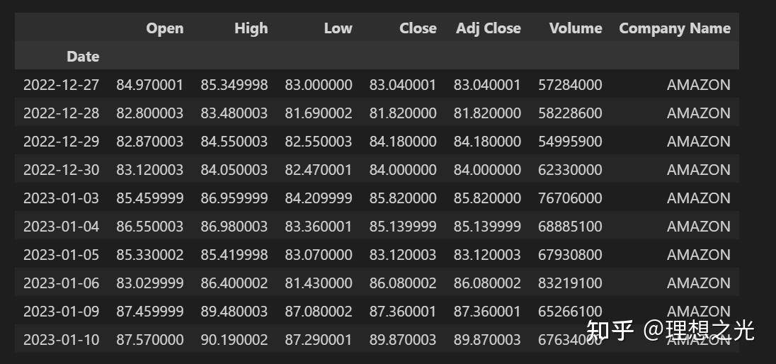
df = pd.concat(companyList, axis=0)
df.tail(10)得到的表格如下图所示:
数据分析
通常采用df.describe()和df.info()来查看数据是否有空值。
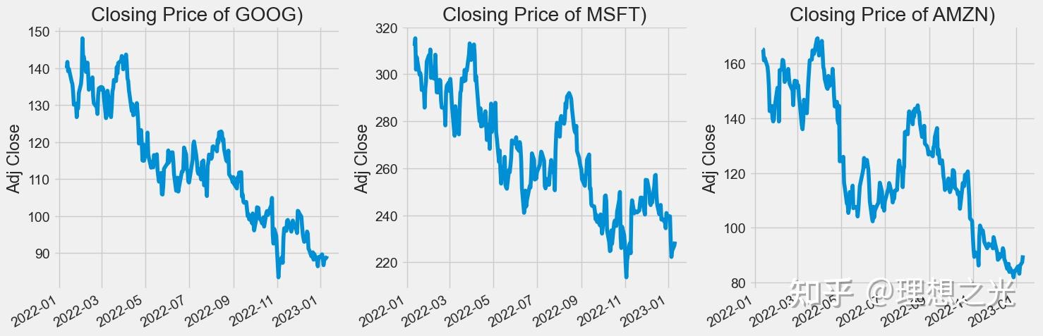
在股票市场中,投资者通常使用收盘价来追踪股票的趋势,下面用matplotlib来查看三个公司的股票趋势。
收盘价
plt.figure(figsize=(15, 5))
plt.subplots_adjust(top=1.25, bottom=1.2)
for i, company in enumerate(companyList, 1):
plt.subplot(1, 3, i)
company['Adj Close'].plot()
plt.ylabel('Adj Close')
plt.xlabel(None)
plt.title(f"Closing Price of {techList[i-1]})")
plt.tight_layout()
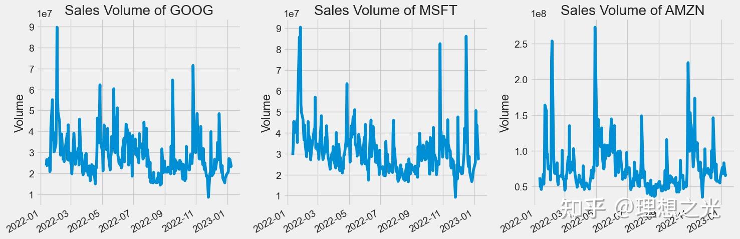
交易量
交易量是指在一段时间内(通常是一天内)易手的资产或证券的数量。例如,股票交易量指的是每日开盘和收盘之间交易的证券股数。交易量以及交易量随时间的变化是技术交易者的重要输入。
# 交易量趋势图
plt.figure(figsize=(15, 5))
plt.subplots_adjust(top=1.25, bottom=1.2)
for i, company in enumerate(companyList, 1):
plt.subplot(1, 3, i)
company['Volume'].plot()
plt.ylabel('Volume')
plt.xlabel(None)
plt.title(f"Sales Volume of {techList[i-1]}")
plt.tight_layout()
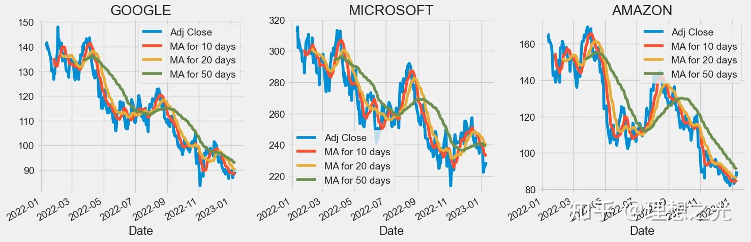
移动平均线
移动平均线 (MA) 是一种简单的技术分析工具,通过创建不断更新的平均价格来平滑价格数据。平均值取自特定时间段,例如 10 天、20 分钟、30 周或交易者选择的任何时间段。
# 移动平均线
maDay = [10, 20, 50]
for ma in maDay:
for company in companyList:
column_name = f"MA for {ma} days"
company[column_name] = company['Adj Close'].rolling(ma).mean()
fig, axes = plt.subplots(nrows=1, ncols=3)
fig.set_figheight(5)
fig.set_figwidth(15)
GOOG[['Adj Close', 'MA for 10 days', 'MA for 20 days', 'MA for 50 days']].plot(ax=axes[0])
axes[0].set_title('GOOGLE')
MSFT[['Adj Close', 'MA for 10 days', 'MA for 20 days', 'MA for 50 days']].plot(ax=axes[1])
axes[1].set_title('MICROSOFT')
AMZN[['Adj Close', 'MA for 10 days', 'MA for 20 days', 'MA for 50 days']].plot(ax=axes[2])
axes[2].set_title('AMAZON')
fig.tight_layout()
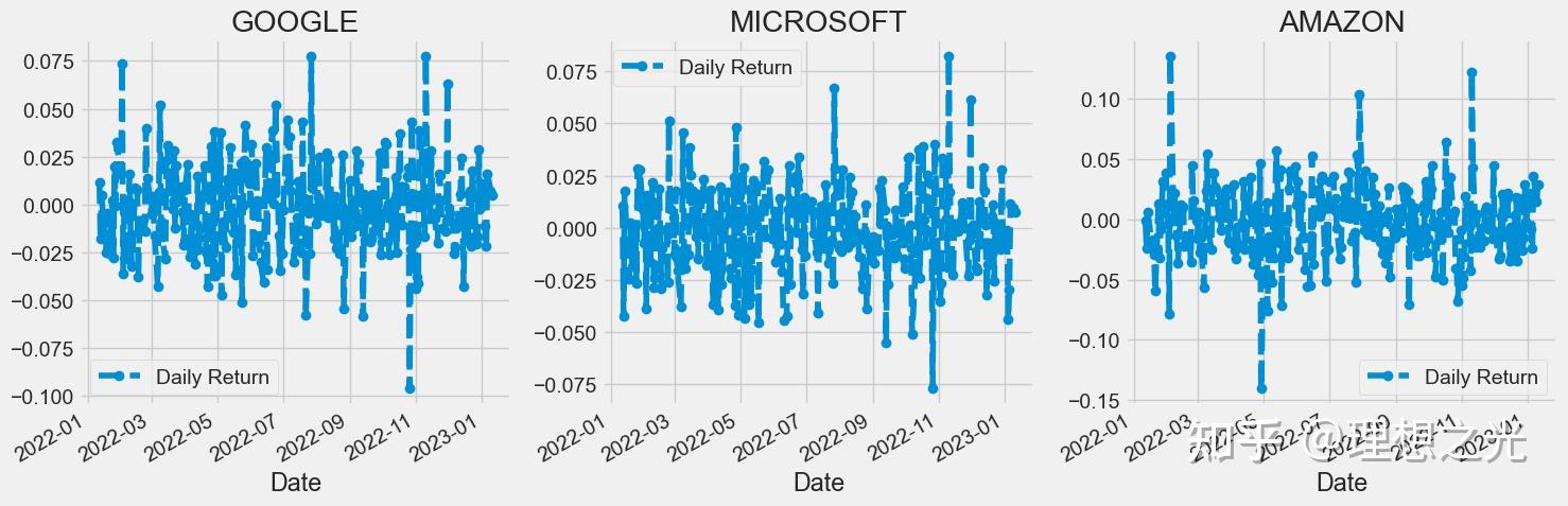
日均收益率
# 日均收益率
for company in companyList:
company['Daily Return'] = company['Adj Close'].pct_change()
fig, axes = plt.subplots(nrows=1, ncols=3)
fig.set_figheight(5)
fig.set_figwidth(15)
GOOG['Daily Return'].plot(ax=axes[0], legend=True, linestyle='--', marker='o')
axes[0].set_title('GOOGLE')
MSFT['Daily Return'].plot(ax=axes[1], legend=True, linestyle='--', marker='o')
axes[1].set_title('MICROSOFT')
AMZN['Daily Return'].plot(ax=axes[2], legend=True, linestyle='--', marker='o')
axes[2].set_title('AMAZON')
fig.tight_layout()
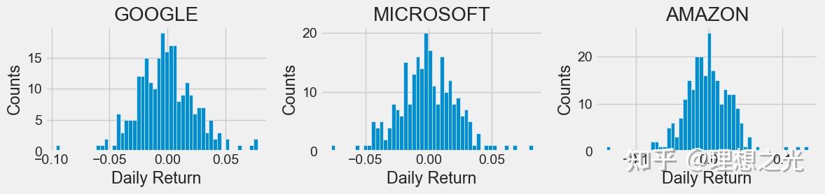
plt.figure(figsize=(12, 3))
for i, company in enumerate(companyList, 1):
plt.subplot(1, 3, i)
company['Daily Return'].hist(bins=50)
plt.xlabel('Daily Return')
plt.ylabel('Counts')
plt.title(f'{companyName[i - 1]}')
plt.tight_layout()
相关性分析
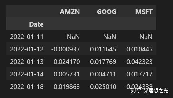
相关性是一种统计量,用于衡量两个变量相对于彼此移动的程度,其值必须介于 -1.0 和 +1.0 之间。相关性衡量关联,但不说明x 是否导致 y ,反之亦然——或者关联是否由第三个因素引起 。 在相关性分析之前,先构建一个DataFrame,其列为各个公司,行为每个公司对应日期的收盘价。
closingDf = DataReader(techList, start, end)['Adj Close']
techRets = closingDf.pct_change()
techRets.head()
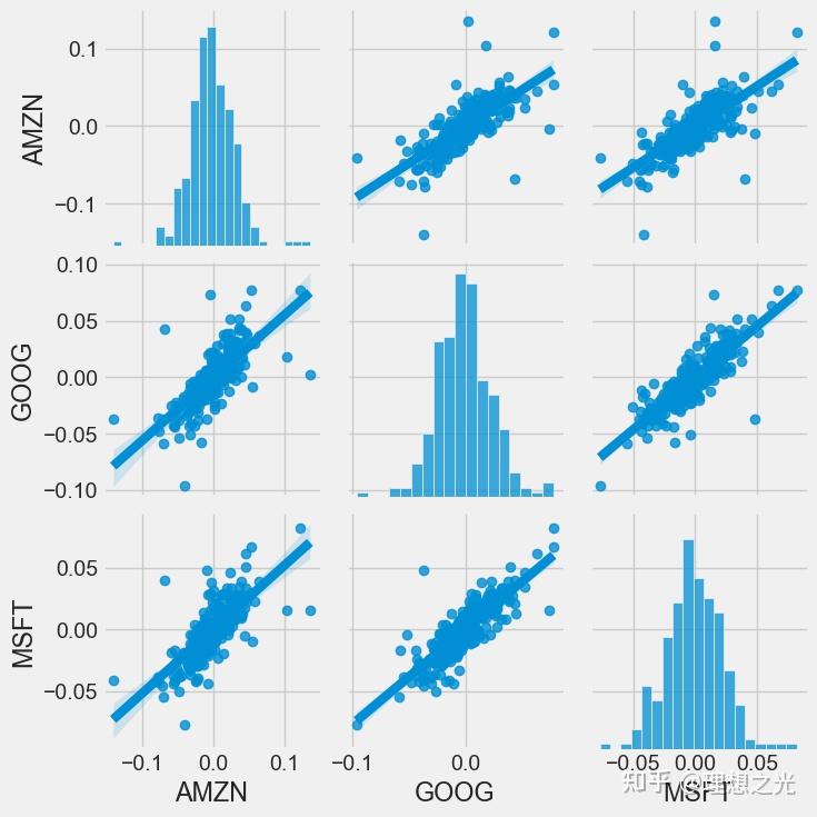
然后用seaborn画出相关性图:
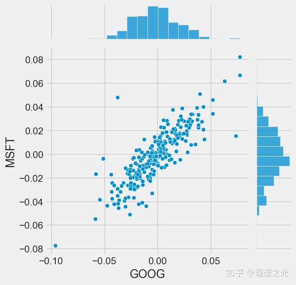
要得到多个列的相关性分析,只需要:
sns.pairplot(techRets, kind='reg')
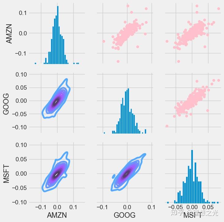
当然,pairplot是一个封装的很好的包,也可以使用PairGrid来自定义布局:
# 自定义布局
retFig = sns.PairGrid(techRets.dropna())
retFig.map_upper(plt.scatter, color='Pink')
retFig.map_lower(sns.kdeplot, cmap='cool_d')
retFig.map_diag(plt.hist, bins=30)
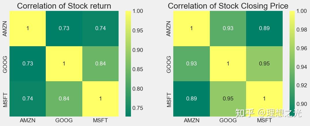
相似矩阵
可以用热力图以及标注数字来查看具体相似度。
plt.figure(figsize=(12,10))
plt.subplot(2,2,1)
sns.heatmap(techRets.corr(), annot=True, cmap='summer')
plt.title('Correlation of Stock return')
plt.subplot(2,2,2)
sns.heatmap(closingDf.corr(), annot=True, cmap='summer')
plt.title('Correlation of Stock Closing Price')
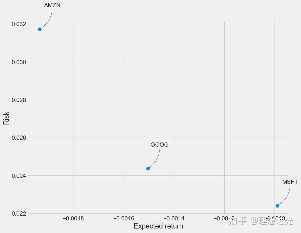
风险衡量
我们有多种衡量风险的方式,其中一种最基本的方式是将预期回报和每日回报的标准差进行比较。
rets = techRets.dropna()
area = np.pi * 20
plt.figure(figsize=(10, 8))
plt.scatter(rets.mean(), rets.std(), s=area)
plt.xlabel('Expected return')
plt.ylabel('Risk')
for label, x, y in zip(rets.columns, rets.mean(), rets.std()):
plt.annotate(label, xy=(x, y), xytext=(50, 50), textcoords='offset points', ha='right', va='bottom',
arrowprops=dict(arrowstyle='-', color='blue', connectionstyle='arc3,rad=-0.3'))
数据预测
在下面的部分将使用LSTM对GOOG公司的收盘价进行预测。
数据分析
获取数据
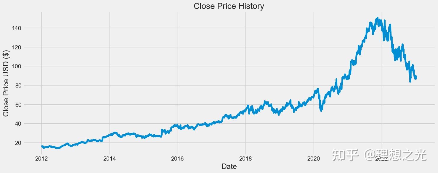
df = DataReader('GOOG', start='2012-01-01', end=end)
df了解数据
画出GOOG收盘价的趋势。
构建数据集
# 创建一个只有收盘价的DF
data = df.filter(['Close'])
# 将DataFrame转换为numpy
dataset = data.values
# 获取行数
lenOfTrain = int(np.ceil(len(dataset) * .95))
lenOfTrain
# 标准化数据
from sklearn.preprocessing import MinMaxScaler
scaler = MinMaxScaler(feature_range=(0,1))
scaled_data = scaler.fit_transform(dataset)
scaled_data
# 创建数据集
trainData = scaled_data[0:int(lenOfTrain), :]
X_train = []
y_train = []
for i in range(60, len(trainData)):
X_train.append(trainData[i-60:i, 0])
y_train.append(trainData[i,0])
# 打印部分查看数据结构
if i == 60:
print(X_train)
print(y_train)
# 转换为numpy
X_train, y_train = np.array(X_train), np.array(y_train)
# 转换数据形状
X_train = np.reshape(X_train, (X_train.shape[0], X_train.shape[1], 1))
# 打印形状
print(f"训练集的形状为{X_train.shape}") 输出为:
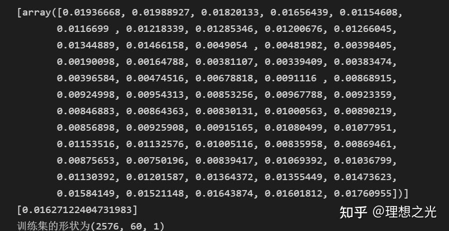
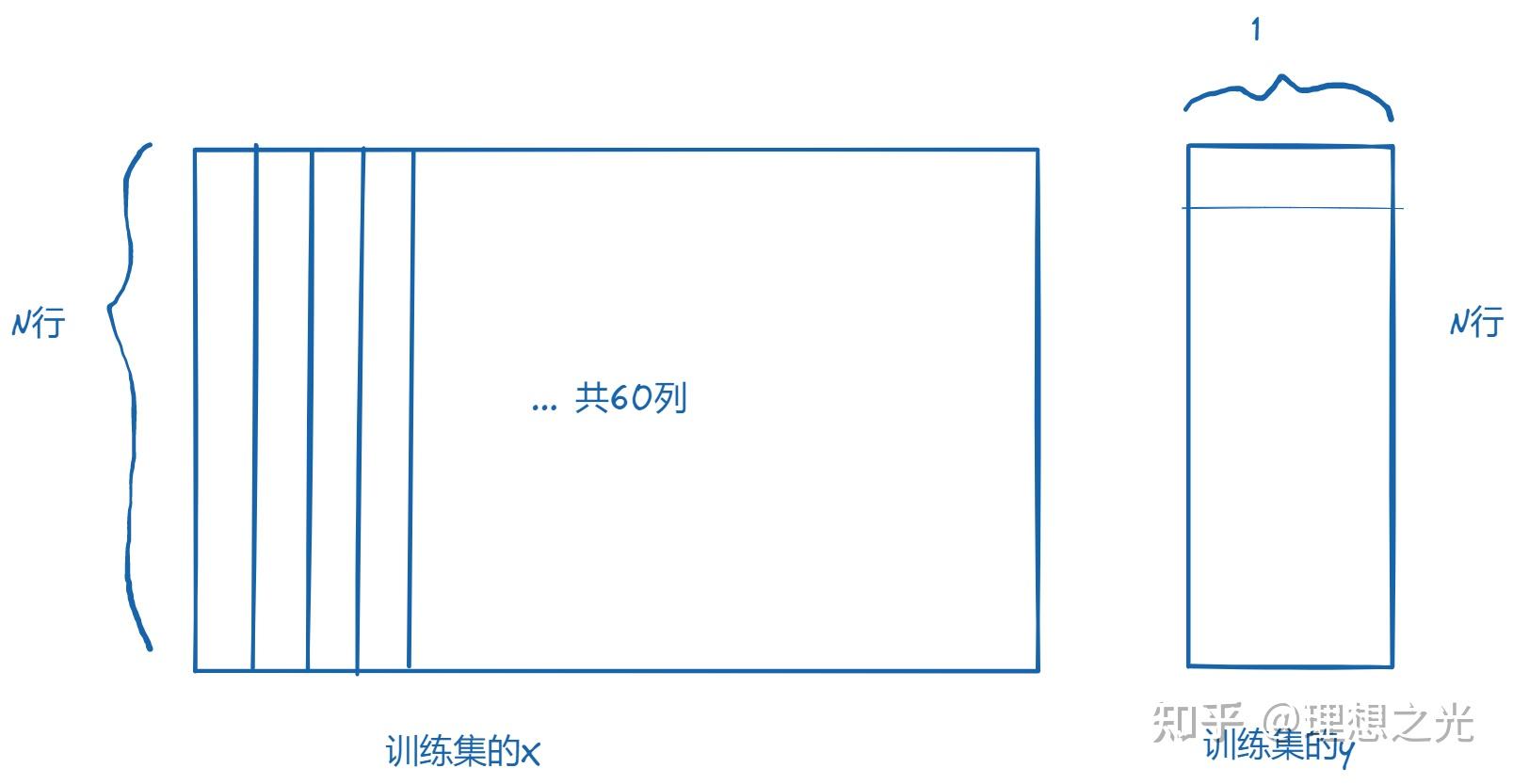
即训练集的X:每个行代表从第61天开始到最后一天,每天有60个列,每个列代表从该天往前推i天。
训练集的y:每个行代表当天的收盘价,只有1列。
构建模型
这里的模型构建使用Keras库(使用前需要安装Tensorflow框架)。
关于LSTM模型,可以查看参考文献中的链接。
model = Sequential()
model.add(LSTM(128, return_sequences=True, input_shape= (x_train.shape[1], 1)))
model.add(LSTM(64, return_sequences=False))
model.add(Dense(25))
model.add(Dense(1))
# 添加优化器和损失函数
model.compile(optimizer='adam', loss='mean_squared_error')
# 训练模型
model.fit(x_train, y_train, batch_size=1, epochs=1)接下来介绍一些核心函数的核心参数,具体细节请查看官方文档:https://keras.io/zh/
keras.layers.recurrent.LSTM(units, activation='tanh', recurrent_activation='hard_sigmoid', use_bias=True, kernel_initializer='glorot_uniform', recurrent_initializer='orthogonal', bias_initializer='zeros', unit_forget_bias=True, kernel_regularizer=None, recurrent_regularizer=None, bias_regularizer=None, activity_regularizer=None, kernel_constraint=None, recurrent_constraint=None, bias_constraint=None, dropout=0.0, recurrent_dropout=0.0)
- units:输出维度
- input_dim:输入维度,当使用该层为模型首层时,应指定该值(或等价的指定input_shape)
- return_sequences:布尔值,默认False,控制返回类型。若为True则返回整个序列,否则仅返回输出序列的最后一个输出
- input_length:当输入序列的长度固定时,该参数为输入序列的长度。当需要在该层后连接Flatten层,然后又要连接Dense层时,需要指定该参数,否则全连接的输出无法计算出来。
下面参考CSDN上的一个博客讲解LSTM的输入输出:
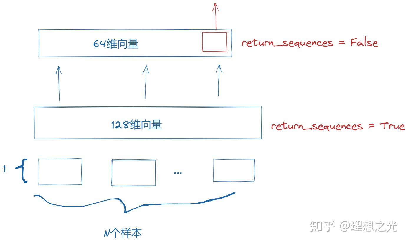
当LSTM是中间层时,必须return_sequences = True,这样才能保证各个层的维度相同。 速度还是很快的,在i9-12900H的电脑上27.5s就完成了。
测试模型
# 创建验证集
testData = scaled_data[lenOfTrain - 60:,:]
X_test = []
y_test = dataset[lenOfTrain:, :]
for i in range(60, len(testData)):
X_test.append(testData[i-60:i, 0])
X_test = np.array(X_test)
X_test = np.reshape(X_test, (X_test.shape[0], X_test.shape[1], 1))
# 预测
predictions = model.predict(X_test)
predictions = scaler.inverse_transform(predictions)
rmse = np.sqrt(np.mean(((predictions - y_test) ** 2)))
rmse查看一下预测的结果:
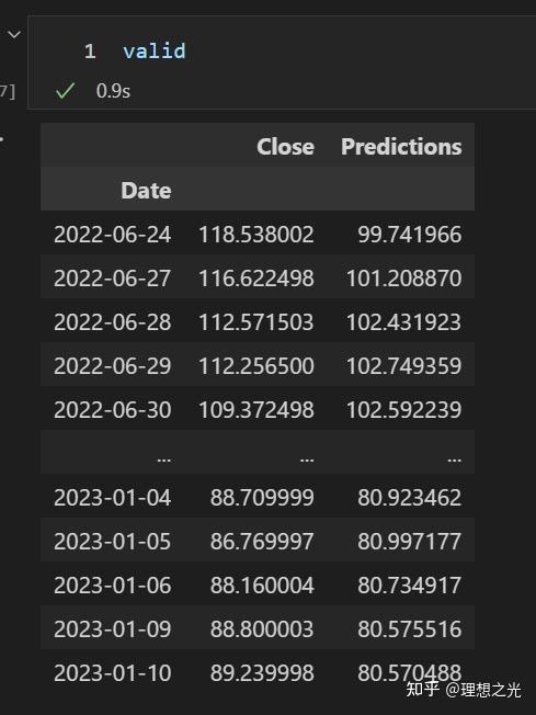
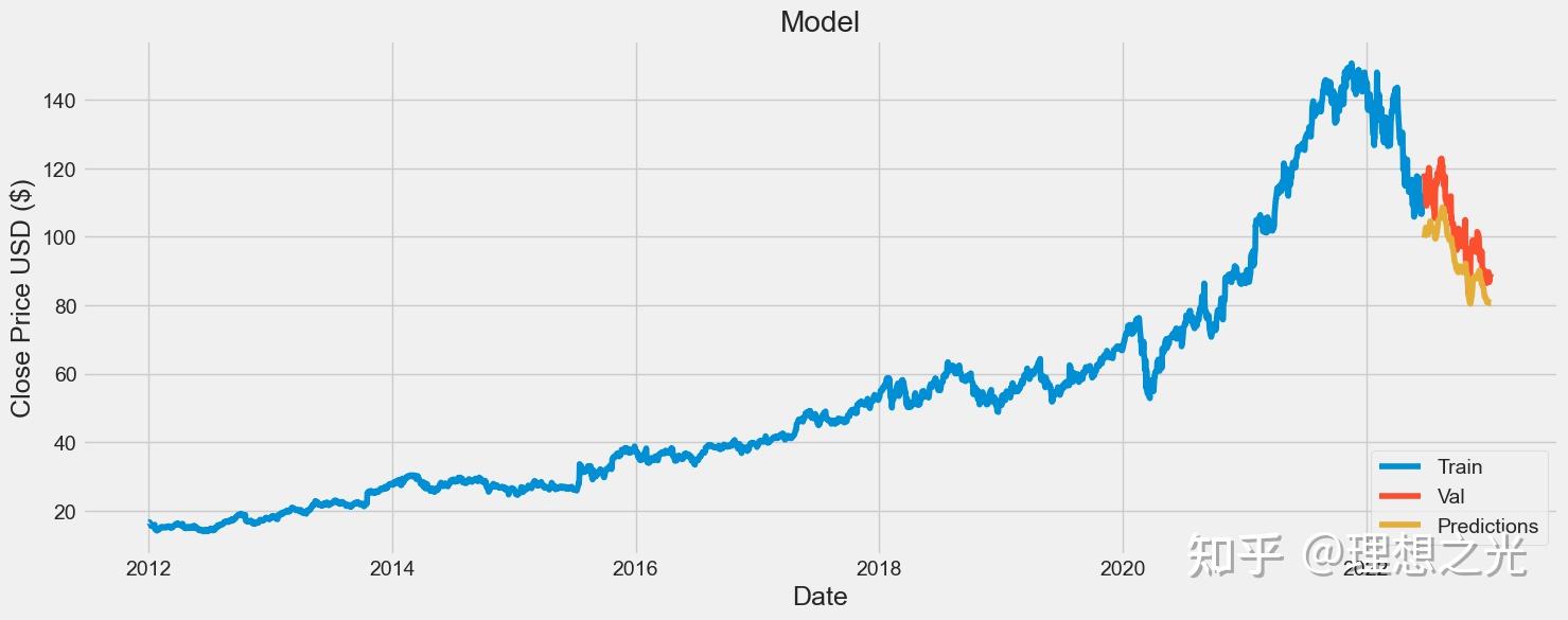
画图可以更清晰看出验证结果和真实结果的差距。
# 画图
train = data[:lenOfTrain]
valid = data[lenOfTrain:]
valid['Predictions'] = predictions
# Visualize the data
plt.figure(figsize=(16,6))
plt.title('Model')
plt.xlabel('Date', fontsize=18)
plt.ylabel('Close Price USD ($)', fontsize=18)
plt.plot(train['Close'])
plt.plot(valid[['Close', 'Predictions']])
plt.legend(['Train', 'Val', 'Predictions'], loc='lower right')
plt.show()
参考文献
[1] https://www.kaggle.com/code/faressayah/stock-market-analysis-prediction-using-lstm/notebook
[2] 在Keras中使用LSTM模型:http://t.csdn.cn/DagYI
[3] LSTM模型: |
|


 发表于 2023-1-18 07:08:32